Deep Neural Network 文章筆記整理
1102 機器學習
Deep Learning 總整理這篇文章是學習時整理的一些筆記,讓自己複習時方便,文章內容為上課之內容整理
深度學習主要是模仿人類神經元的運作,分為DNN, CNN及RNN…等
本篇主要在講述DNN,若是想看別的,可以點擊下方按鈕喔~
DNN 介紹
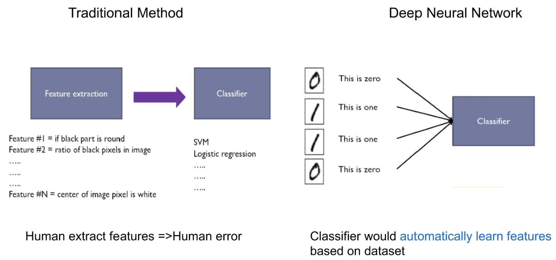
在傳統的方法裡,是先經由人類提取特徵後在交由機器去學習這些特徵,在現在的深度學習中,機器除了要學習特徵外,也要學習如何提取特徵
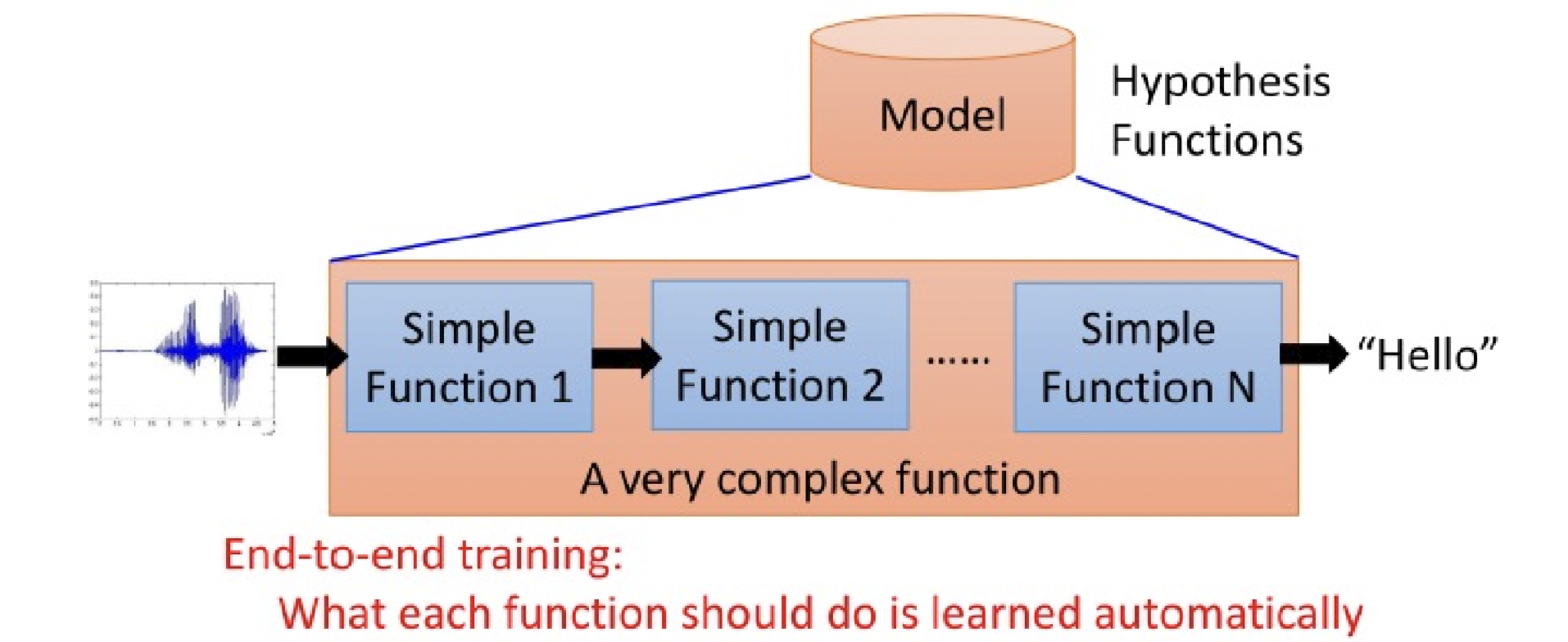
each of the function can learn from data, less engineering labor, but machine learns more
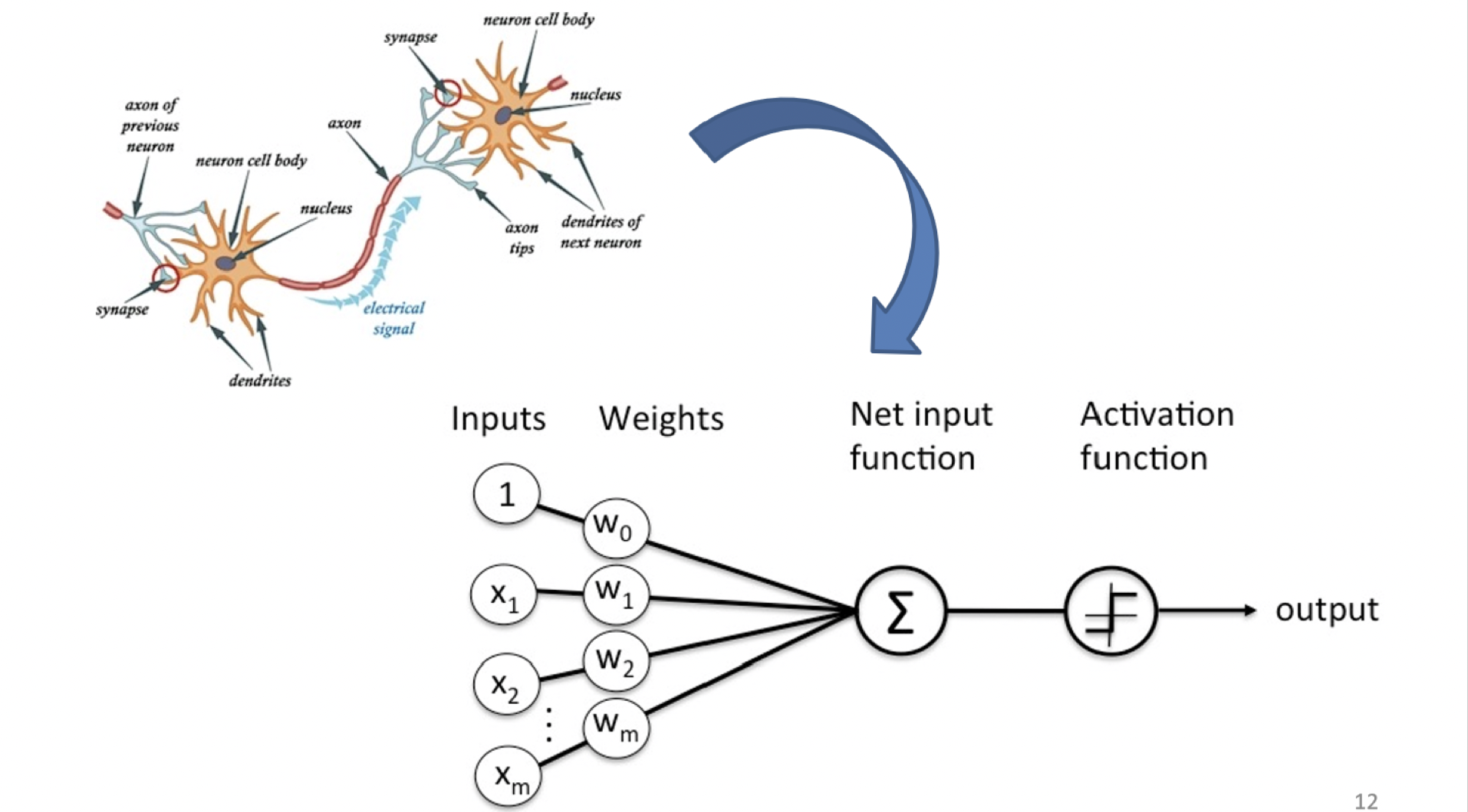
相信大家國中的時候都認識過人體的神經系統。假設我們現在要判斷一個人是男是女。我們的眼睛、耳朵等等受器會將接收到的訊息,例如這個人的五官輪廓、聲音高低、身高體重等等,藉著神經系統傳遞到大腦,大腦便會得出是男是女的預測。讓電腦學會接收訊息並判斷預測,即是人工智慧的終極目的。
神經系統的基本元件,意即神經元(Neuron),構造如圖。感知訊息從上一個神經元經由突觸傳進來,再由樹突整合後傳遞至細胞體。若細胞體形成動作電位,則會將訊息藉由軸突傳遞出去,進入下個神經元 [2]。好的這邊看過就能忘了,我最討厭生物。
而電腦科學家有了這麼一個想法:仿造神經元,再將之串連再一起,形成神經網絡(Neural Network)。這個早在 1957 年即被發明的人工神經元,稱為 Perceptron(感知器),也是而後 Neural Network 與 Deep Learning 的開端。reference
但因為人類的神經網路過於複雜,為了方便電腦模擬因此簡化了一下,將神經元分成多層次,通常會有一個輸入層、一個輸出層加上多個隱藏層。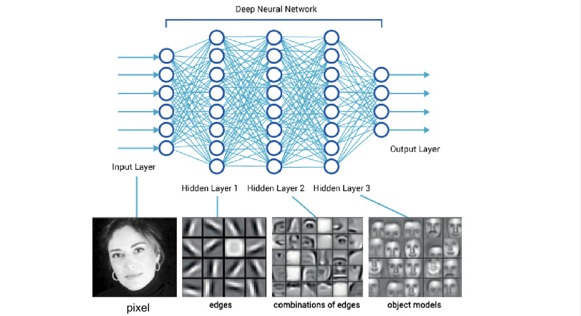
Perceptron 介紹
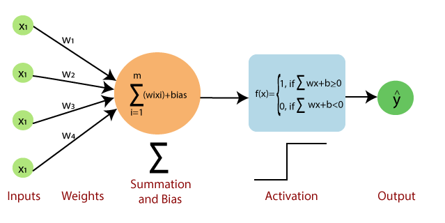
Perceptron對應到的人類神經元的構造有:(以分辨男生女生來說)
- Inputs: 像是人類感官所接收到的訊息,可以有多個特徵,例如聲音高低、五官輪廓
- Weights: 可以想像成是每個接收到的特徵對決定結果的幫助程度,例如在分辨分辨男女上,聲音高低比五官輪廓更能分辨男女
- Bias: 像是男女判斷的標準,前面將所有特徵綜合起來得到一個評分,再拿評分和標準來比較
- Activation: 依據「評分」和「標準」來判斷最終結果的函數,例如評分高於標準為男生、低於為女生等
- Output: 分辨出來的結果
在以上的參數中,weight和bias是參數,我們的目標就是要調整這些參數(也就是訓練模型),讓最終的結果越準確越好。
Perceptron經過運算後將結果輸出到其他神經元,作為其他神經元的輸入,漸漸演變為下圖,也就是我們熟悉的神經網路,每一層都有很多神經元(neuron),上一層的output就是下一層的input,最終得出一組final output
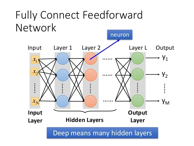
if the number of hidden layer > 1, we call it ‘deep’neural network
Perceptron 運算
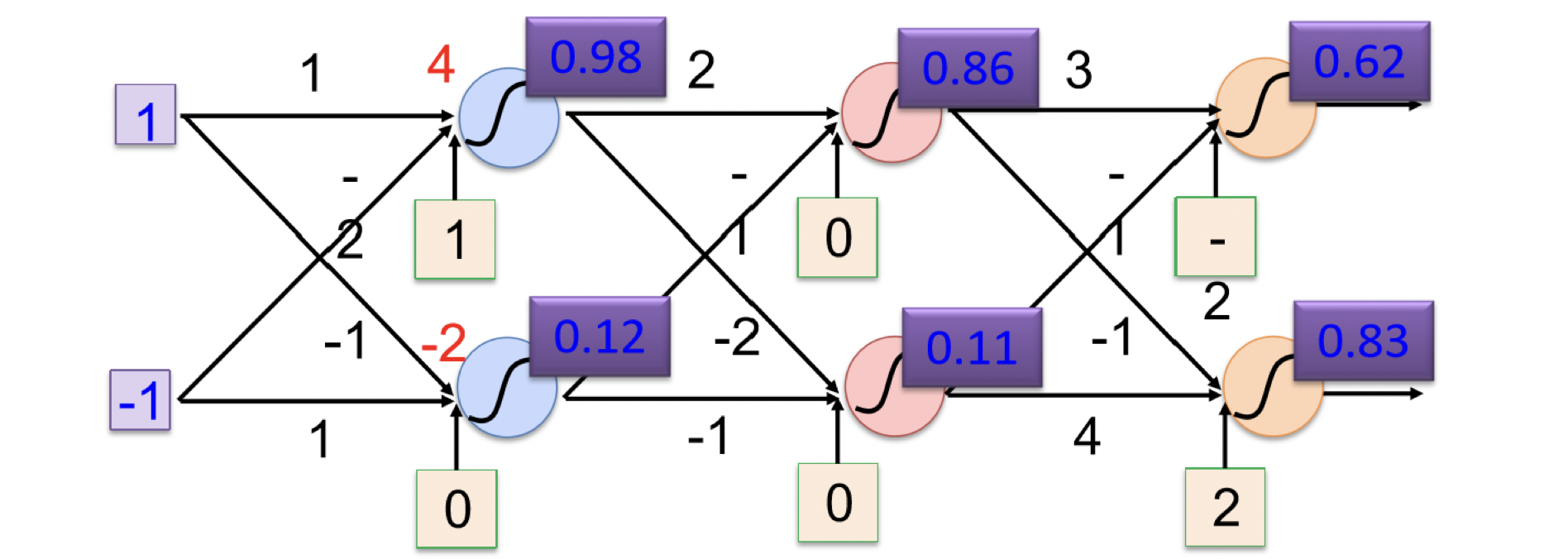
講完了架構,那在每個神經元內又是如何運算後將結果輸出的呢?
我們可以將它比喻做NAND gate,在一系列思考後(如此如此這般這般),可以得知當w1=-1, w2=-1, threshold=-1.5, b=0時,輸入的x1, x2在運算後會完全符合輸出的output,這就是我們要的結果(像是在輸入一堆貓狗圖片後,經過訓練算出一堆w, b,而在這些w,b的組合下,我們可以得到我們要的輸出)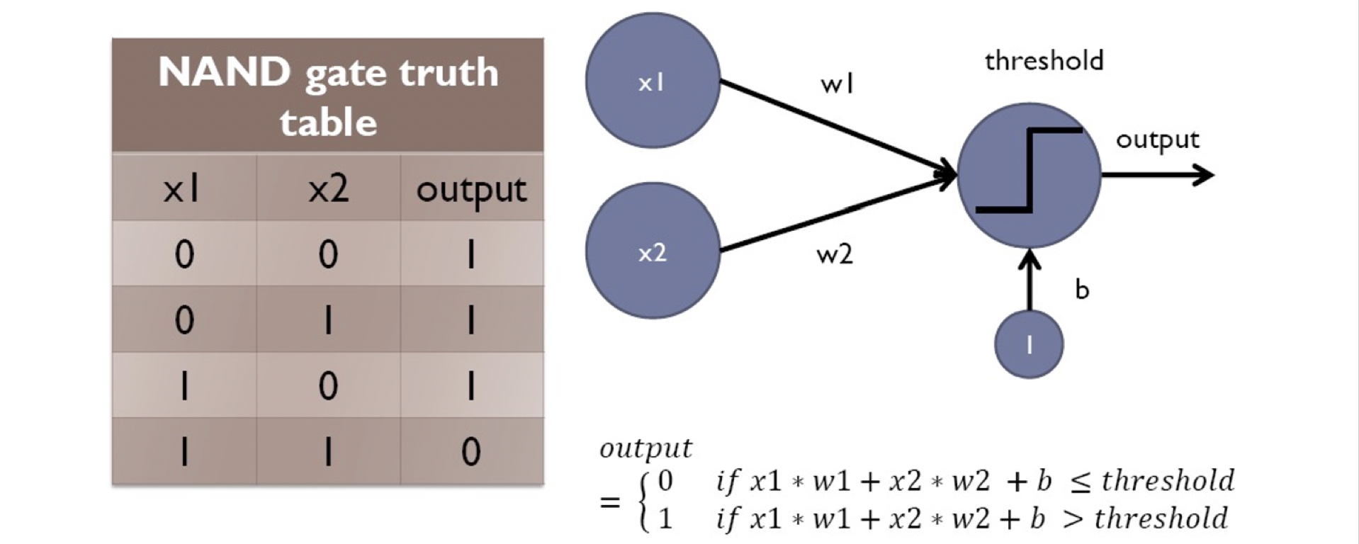
下圖為範例運算圖片
The steps of training Model
no matter which NN, the steps are the same
- prepare dataset
- build model
- define loss
- optimization
Prepare Dataset
在這個階段,我們需要準備所有需要的資料,像是將資料集分成train, test, validation,或是encoded label(one-hot encoding)
關於train, test, validation資料集的差別與用途,可以看另一篇文章
Dataset- spilt part of training data as validation data –> cross validation
- using training data to train model
- using validation data to validate model and modify model
- after modifying model many times, best model is uilt
- using test data to test model
- there are public test data and private data
- the difference of test data and validation data is we don’t use test data to modify model, test data only let us know the model performance under real scenario
Build Model
model overview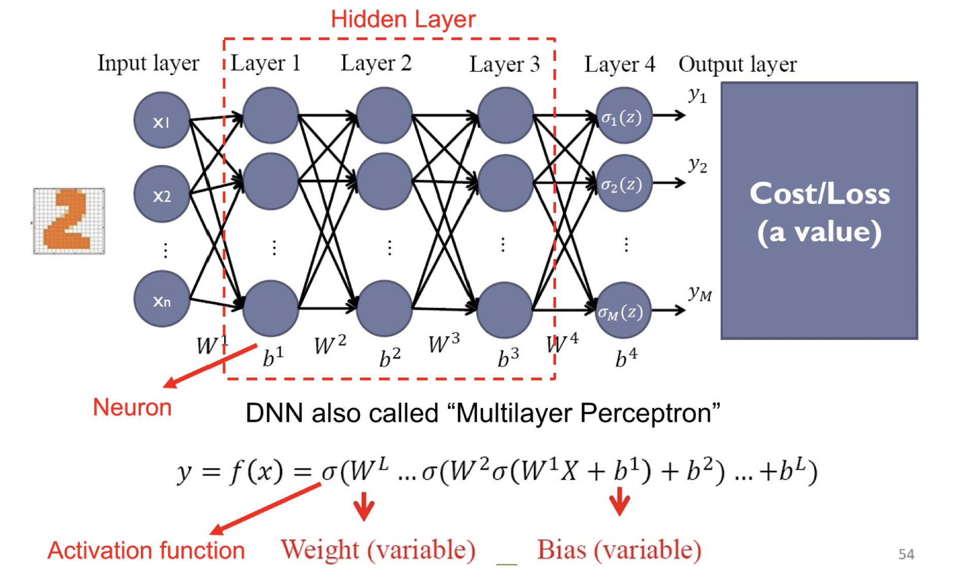

parameter intialization
- the most simple way are
- set all them to zero(sometimes will fail)
- use random normal distribution with zero mean and small standard deviation
- in complex model, it is very important to find better way to initialize parameters
activation function
- given NN non-linear property
- can be regarded as on and off
- usually we use ReLU as first try on building neural network
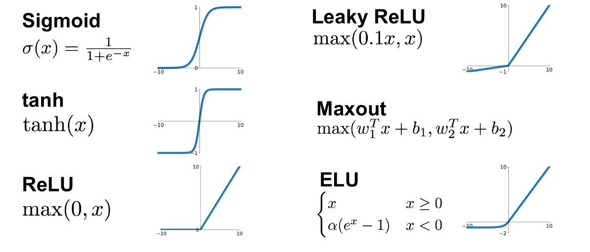
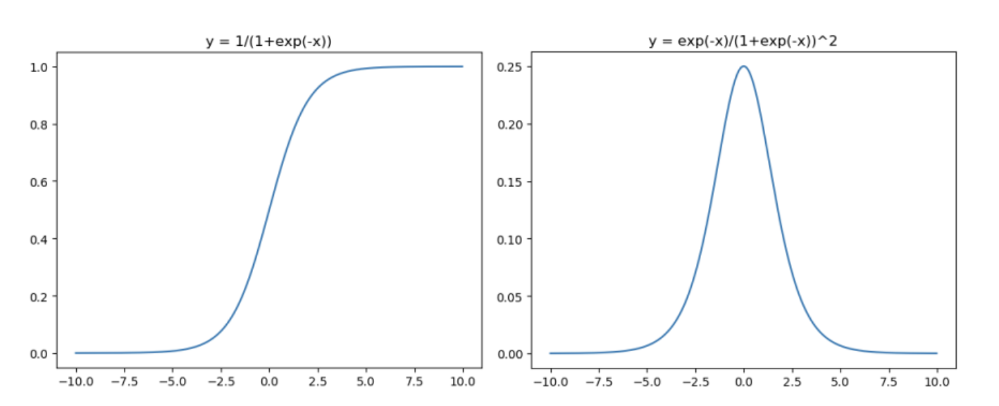
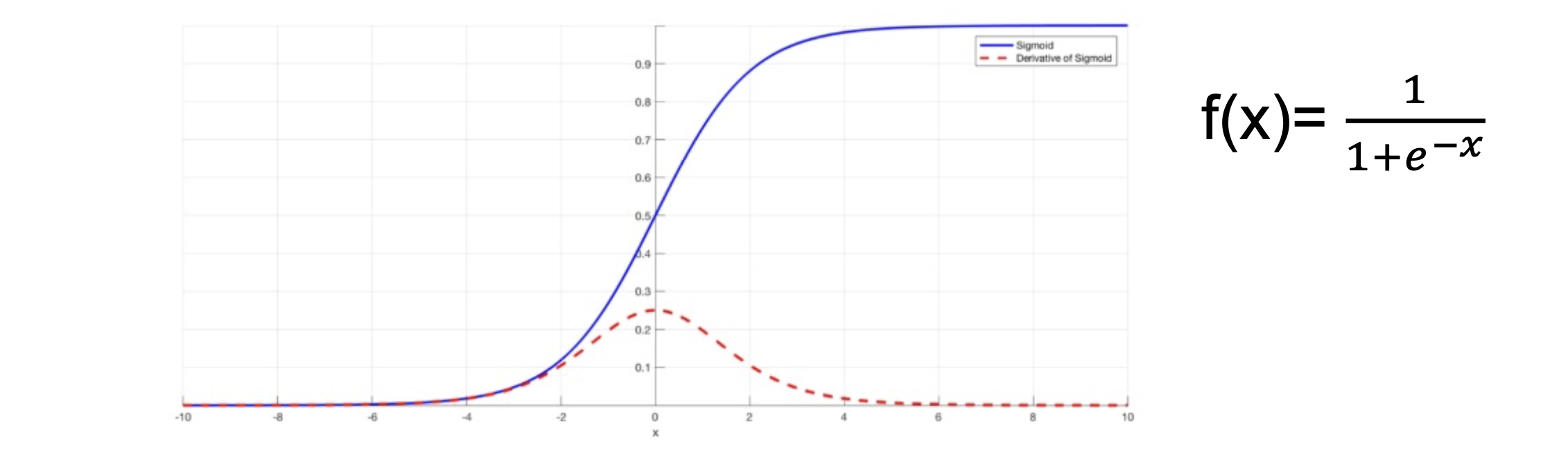
Sigmoid
- the sigmoid function exists between 0 to 1
- therefore, it is especially used for models where we have to predict the probability as an output
- since probability of anything exists only between the range of 0 and 1, simoid is the right choice
sigmoid函數是使用範圍最廣的一個函數,具有指數函數的形狀,他會把一個實數壓縮到0~1之間
不過他存在兩個缺點:
- 有飽和性,在兩側梯度會逐漸趨近於零(類似於神經元死亡概念)
- output的均值不為0,這是不可取的,因為這會導致後一層的的神經元將得到的非0結果都輸入,而若是x(輸入)大於0,且因為f = wx + b,則在反向傳播過程中要馬w都往正向更新,要馬都往負向更新,會導致收斂的非常緩慢
Tanh
- tanh is also like logistic sigmoid but better
- the range of the tanh function is from -1 to 1
Tanh是雙曲函數中的一個,正切函數是非常常見的激活函數,與sigmoid相比,他的輸出均值為0,讓他的收斂速度比sigmoid要來的快,不過他還是和sigmoid一樣會有梯度消失的問題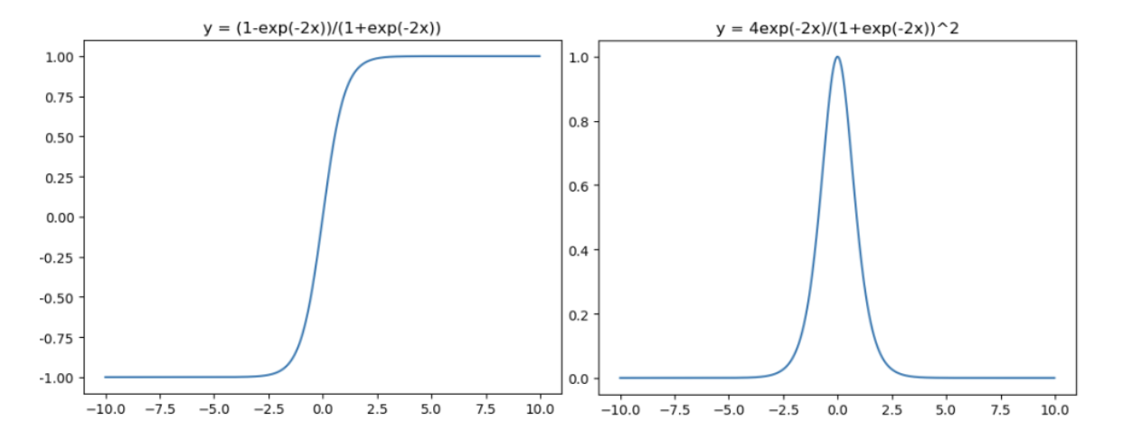
ReLU
- ReLU is half rectified from buttom
- the ReLU is used in almost all the convolutional neural metworks or deep learning: fast to compute / solve vanishing gradient problem
因為Sigmoid函數和tanh的梯度消失缺點,提出了ReLU函數
ReLU被稱為修正線單元,是近年較受歡迎的激活函數,無飽合區且收斂快,計算也簡單,不過有時候會比較脆弱,如果變數的更新太快,還沒有找到最佳值,就進入小於零的分段就會使得梯度變為零,無法更新直接死掉了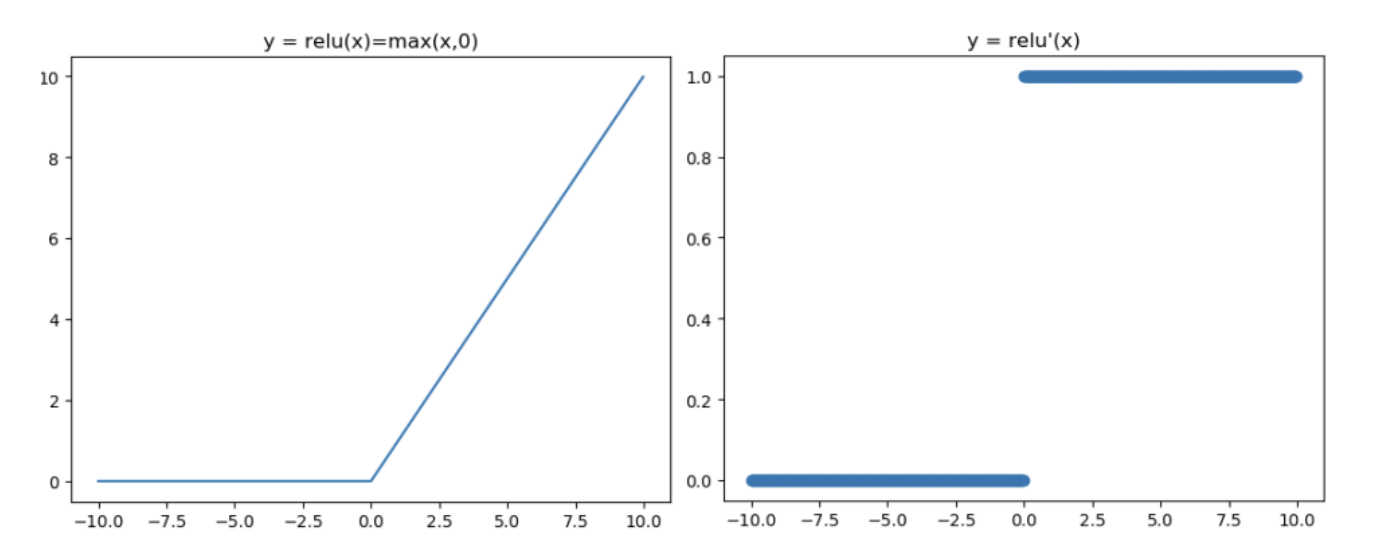
因為ReLU是線性的,而sigmoid和tanh是非線性的,故他有以下特點:
- 解決了梯度消失問題
- 算方便,求導方便,計算速度非常快,只需要判斷輸入是否大於0
- 收斂速度遠遠大於 Sigmoid函數和 tanh函數,可以加速網路訓練
不過因為ReLU也有以下缺點
- 因為負數都為零,故會導致神經元無法激活,即死亡不可逆(有兩種可能導致,第一為一開始初始化時,第二為learning rate 太高,參數更新太大)
- output的均值不為0
關於ReLU在0這點不可導的問題,簡單來說就是直接視為0,詳細解釋可以見👉https://codingnote.cc/zh-tw/p/176736/
Leaky ReLU
- solve dying ReLU problem
- the leak helps to increase the range of ReLU of the ReLU function
- when a is not 0.01 then it is called parametric ReLU
- therefore the range of the Leaky ReLU is -infinity to infinity
為了解決死亡神經元的問題,就將原本前半段從0改為ax(a通常為0.01),Leaky ReLU有ReLU的所有優點,外加不會有 Dead ReLU 問題,但是在實際操作當中,並沒有完全證明Leaky ReLU總是好於ReLU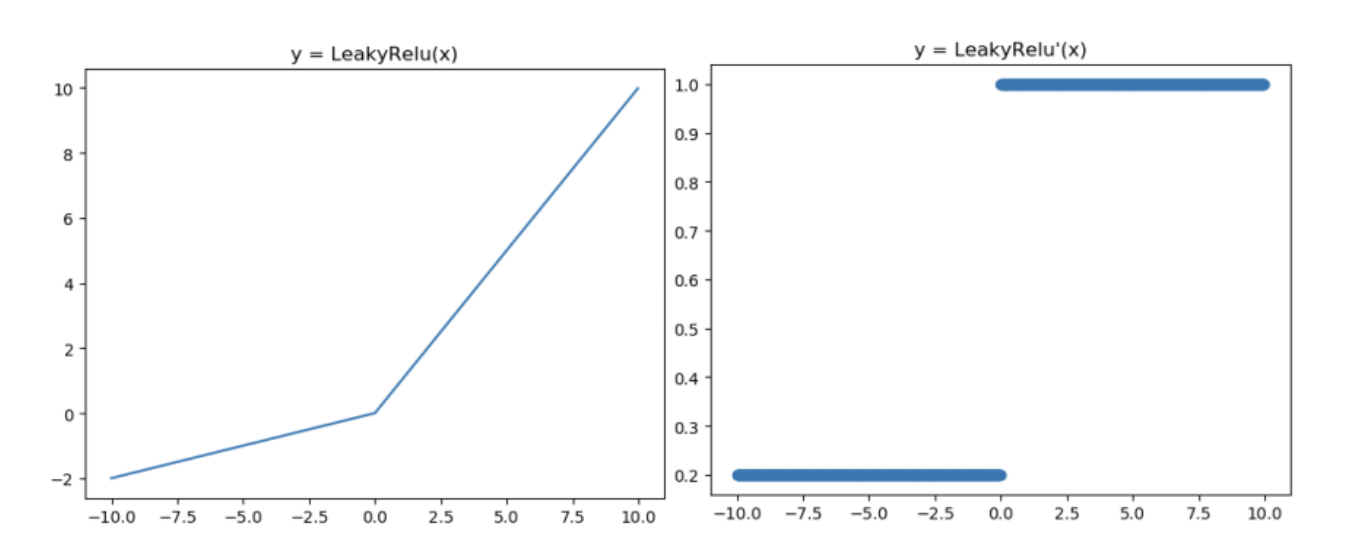
ELU
- exponential linear
- similar to leaky ReLU, ELU has a small slope for negative values
- instead of a straight line, it uses a log curve
融合了Sigmoid和ReLU,左側具有軟飽和性,右側無飽和性,右側線性部分使得ELU緩解梯度消失問題,而左側軟飽能夠讓 ELU 對輸入變化或雜訊更魯棒。因為函數指數項所以計算難度會增加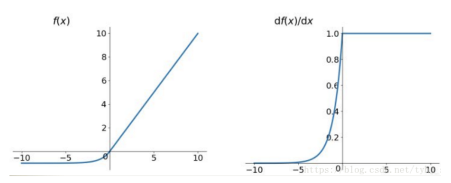
ELU 也是為了解決 ReLU 存在的問題而提出,顯然,ELU有 ReLU的基本所有優點,以及不會出現Dead ReLU 問題,輸出的均值接近0,它的一個小問題在於計算量稍大,類似於 Leaky ReLU,理論上雖然好於 ReLU,但是實際使用中目前並沒有好的證據 ELU 總是優於 ReLU
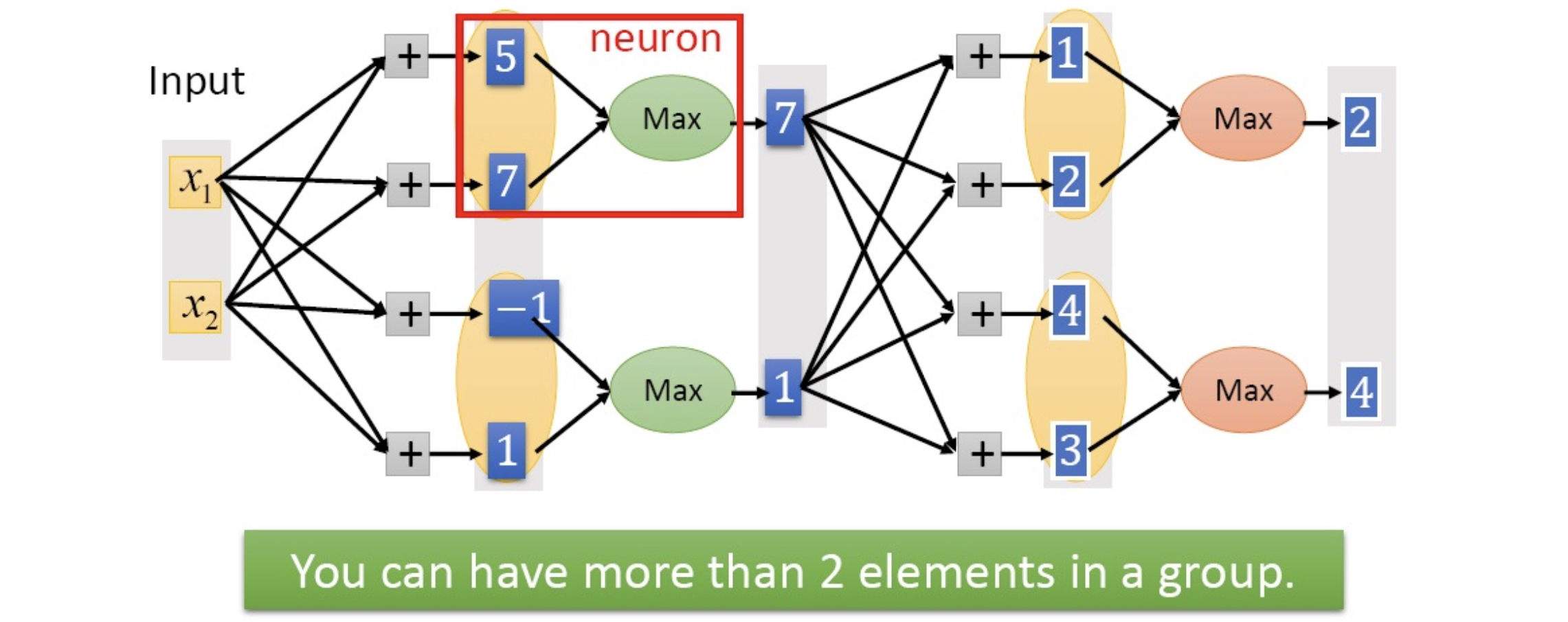
Maxout
在一層同時訓練n組的w,b參數,然後選擇激活值最大的作為下一層神經元的激活值,這個max(Z)函數即充當了激活函數
Define Loss
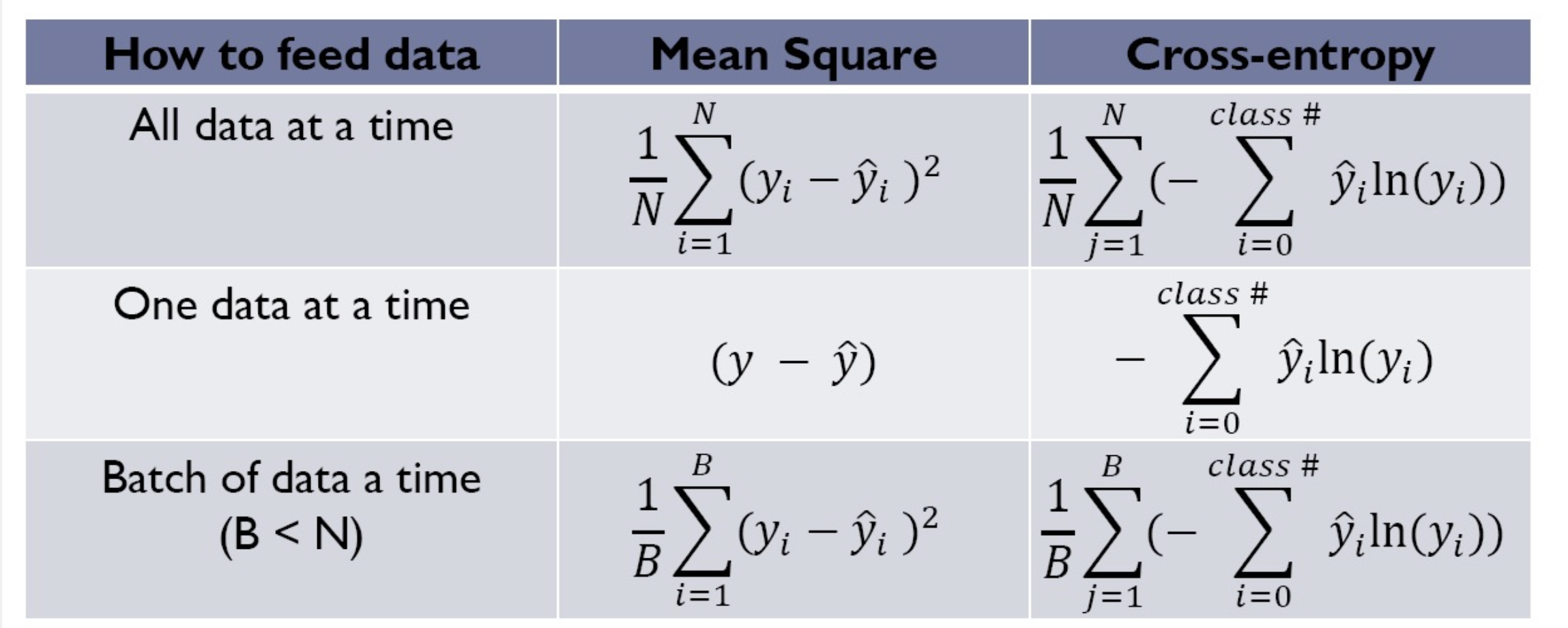
- there are many kinds of loss function
- we will introduce two loss function in DNN: mean-square / cross-entropy
Mean Square
就是我們常見的那個啦~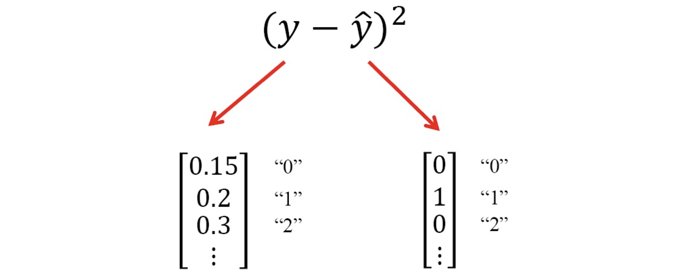
Cross-entrpoy
詳細介紹見下面連結拉!
Entrpoy- measurement on the difference between two probability distribution
- difference distribution apply on entropy
- cross-entropy is greater than entropy
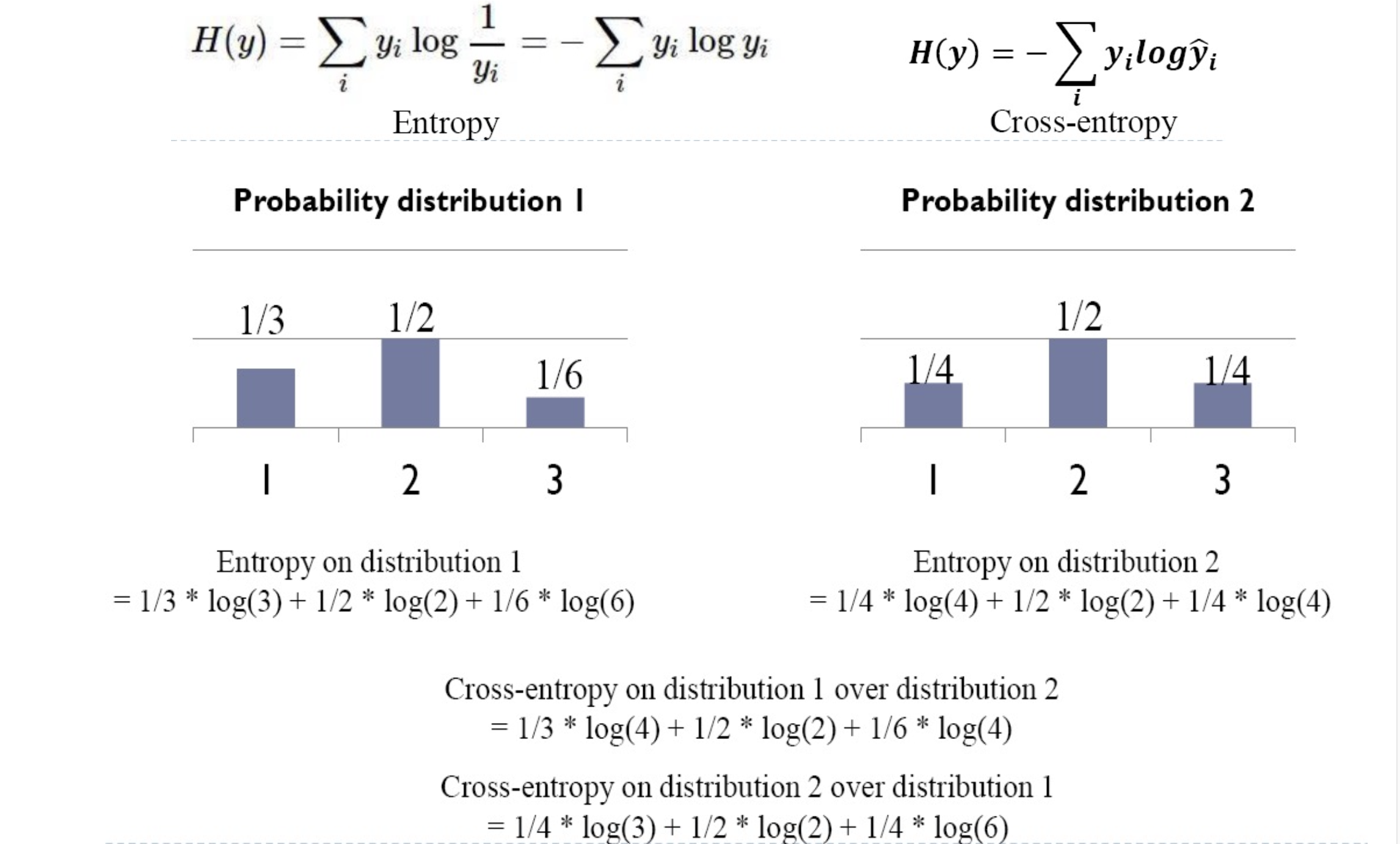

cross-entropy usually come with softmax layer in NN, softmax function squash all of elements in vector to [0, 1]
Summary
Optimization
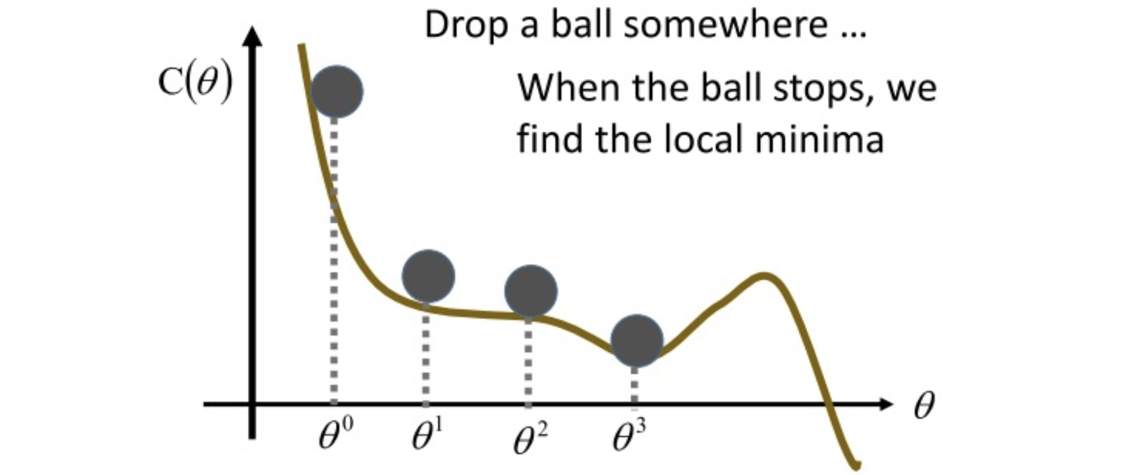
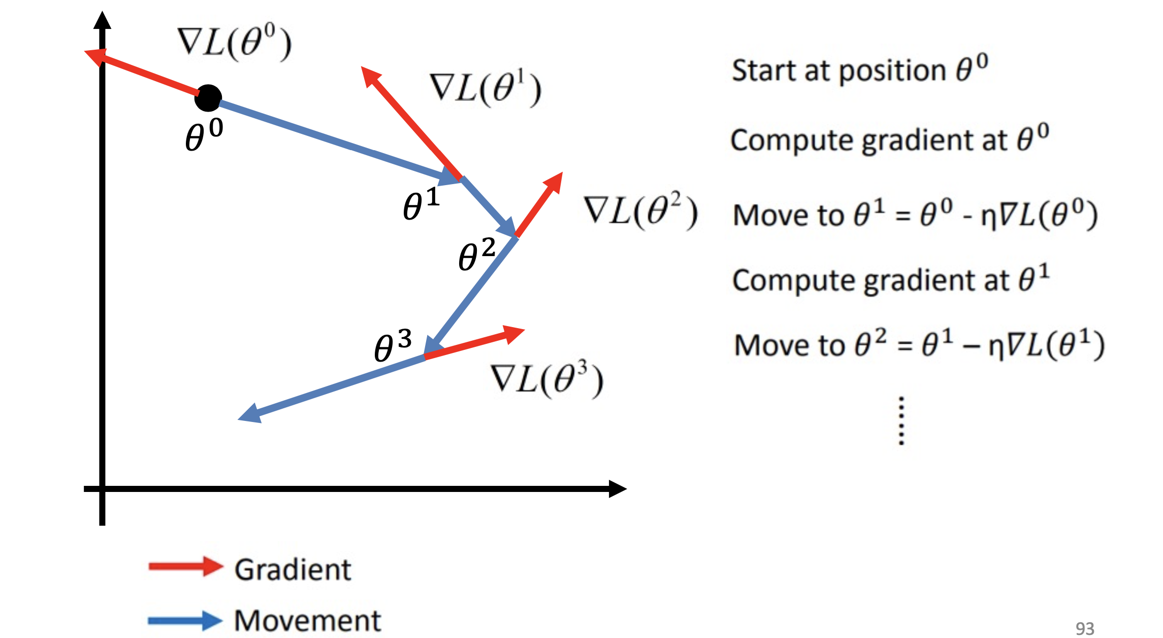
Gradient Descent
就像我們找下山的路一樣,找到向下的路,在數學上我們可以用微分的方式求取斜率,並沿著下坡路慢慢找到最低點,直到微分後為零,就認為是最佳解了
想了解Back propagation的可以跳到另一篇文章~Back Propagation 是什麼?
Increase the performance of optimization
Tune learning rate
The Drawback of Gradient Descent
learning rate would not decay over time, direction of learning rate is fixed
如下圖綠線問題 –> adaptive learning rate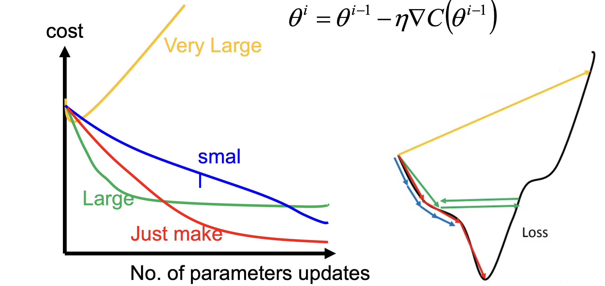
因此如何找到最佳學習率是很重要的議題,加上之前提過的 Gradient Descent 擁有學習率是固定的缺點,所以這邊主要介紹自適應學習率的演算法: Adagrad
adaptive learning rate
- popular and simple ides: reduce the learning rate by some factor every few epochs: after several epochs, we are close to the destination, so we reduce the learning rate
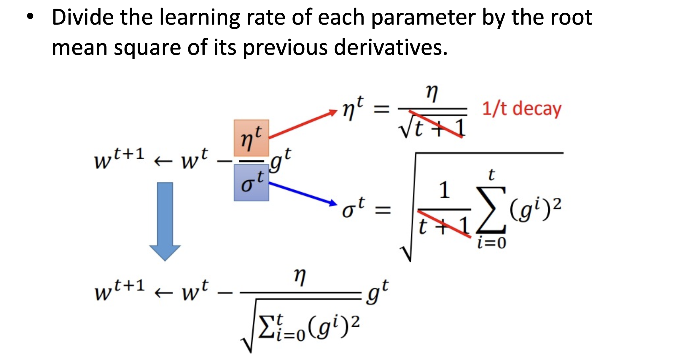
- learning cannot be one-size-fits-all: give different parameters different learning rates –> Adagrad
Adagrad
Adagrad 針對每個參數客制化的值,對學習率進行約束,依照梯度去調整學習率。優點是能加快訓練速度,在前期梯度較小時(較平坦)能夠放大梯度,後期梯度較大時(陡峭)能約束梯度,但缺點是在訓練中後段時有可能梯度趨近於 0,而過早结束學習過程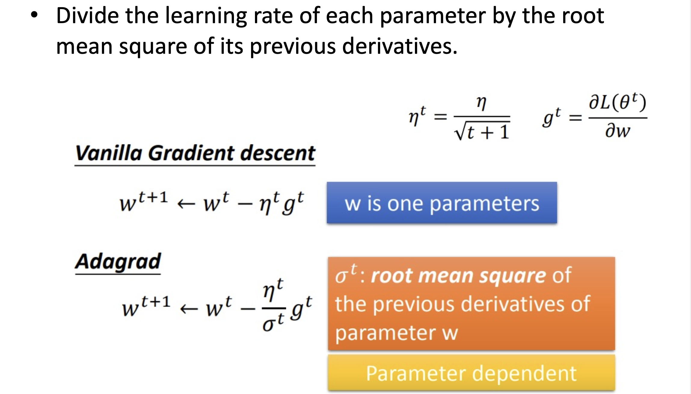
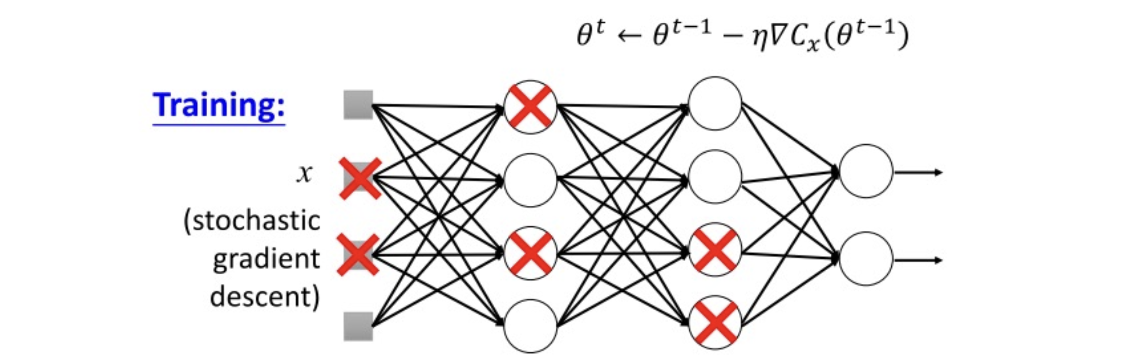
Stochastic gradient descent
GD 是一次用全部樣本去計算損失函數的梯度更新一次參數。
SGD 是一次跑N個樣本然後算出一次梯度的平均後就更新一次,而這些拿來更新梯度的樣本是隨機抽取的,因此被稱為隨機梯度下降法。
Note: 如果有跑過open source API的都會知道需要設定batch size這件事,這件事就是在設定小批次的樣本數。後續方法幾乎都用mini-batch方式作學習。reference
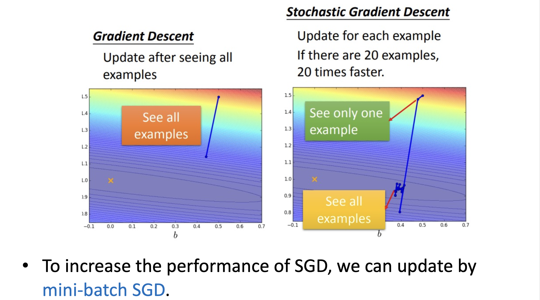
SGD缺點是在當下的問題如果學習率太大,容易造成參數更新呈現鋸齒狀的更新,這是很沒有效率的路徑
Stochastic Gradient Descent and Mini Batch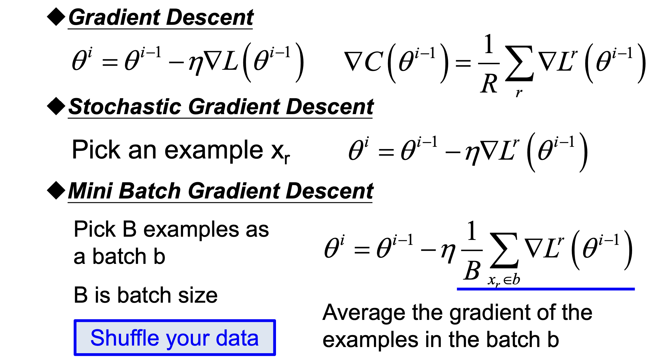
Stochastic Gradient Descenta with Momentum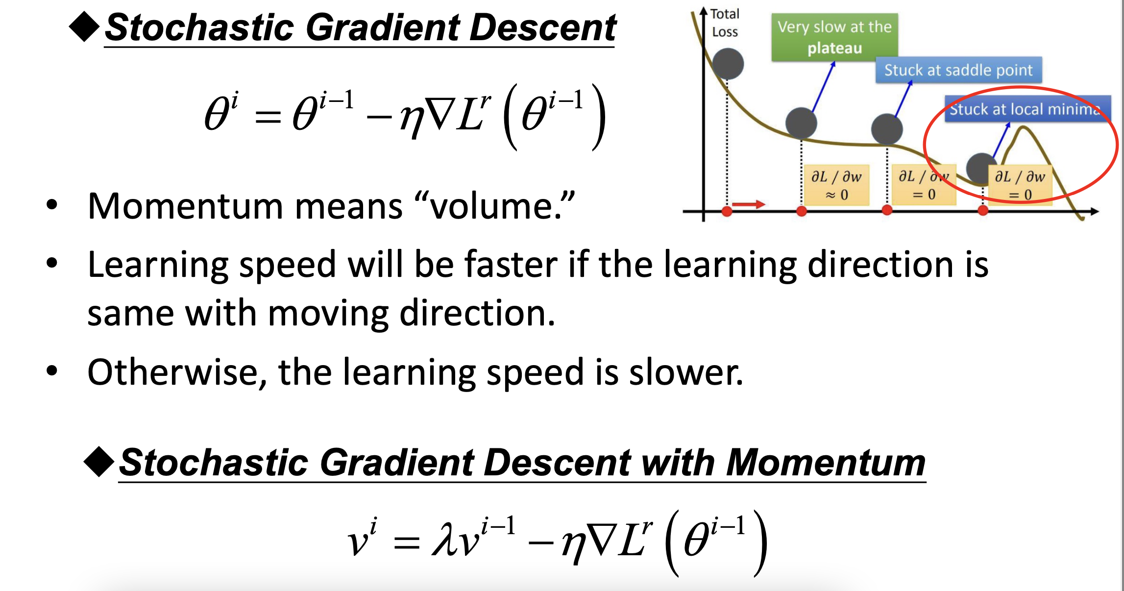
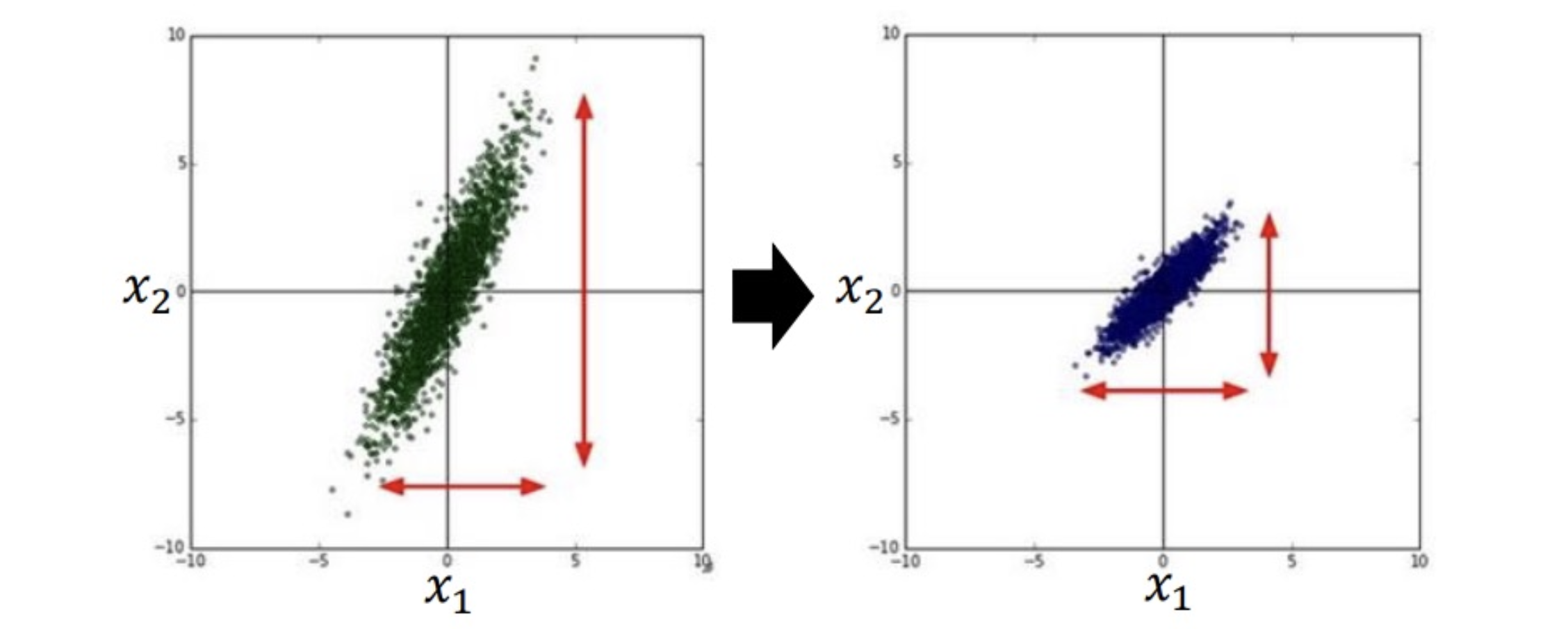
Feature scaling
總結:
Problem in early day of DNN
- Hardware issue: need faster GPU
- Data issue: hard to collect
- Activation function: gradient vanishing
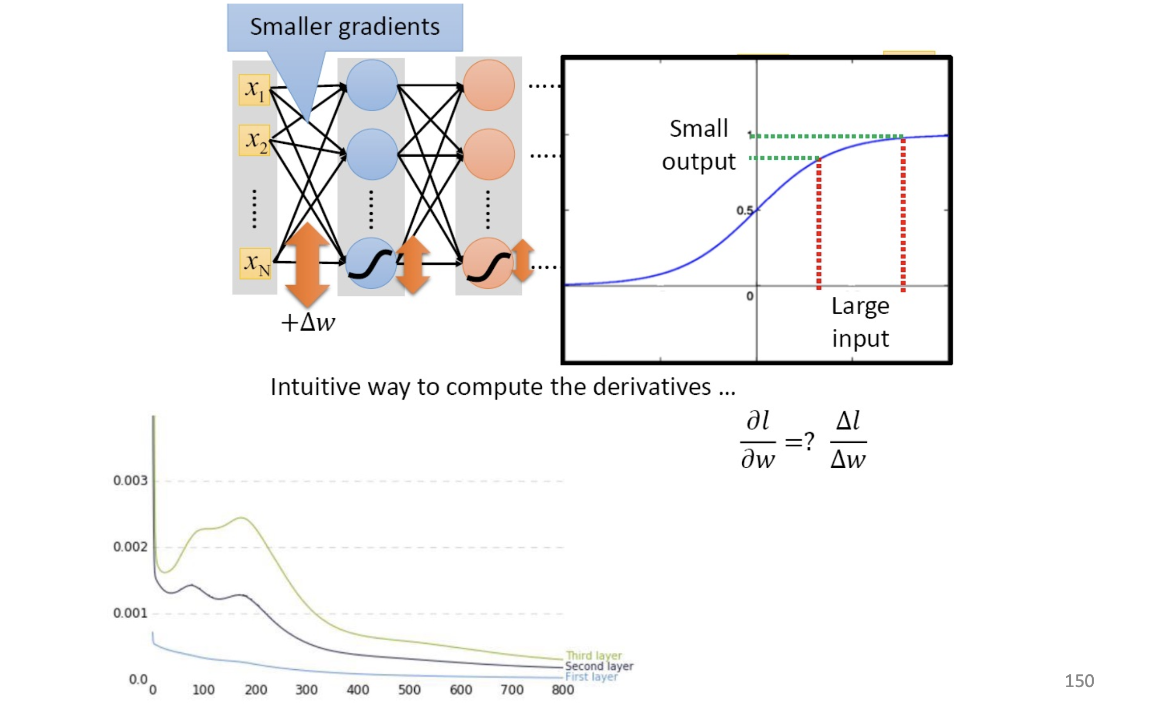
Gradient vanishing problem
因為早期用的激活函數是sigmoid 故會遇到梯度消失的問題(因為sigmoid導數最大為0.25)
- the gradient of front layer is smaller the the back layer
- updating slow and slow…
–> vanishing gradient problem
解決辦法:
- change the activation function: ReLU
- change the activation: Maxout
Problem of Overfitting
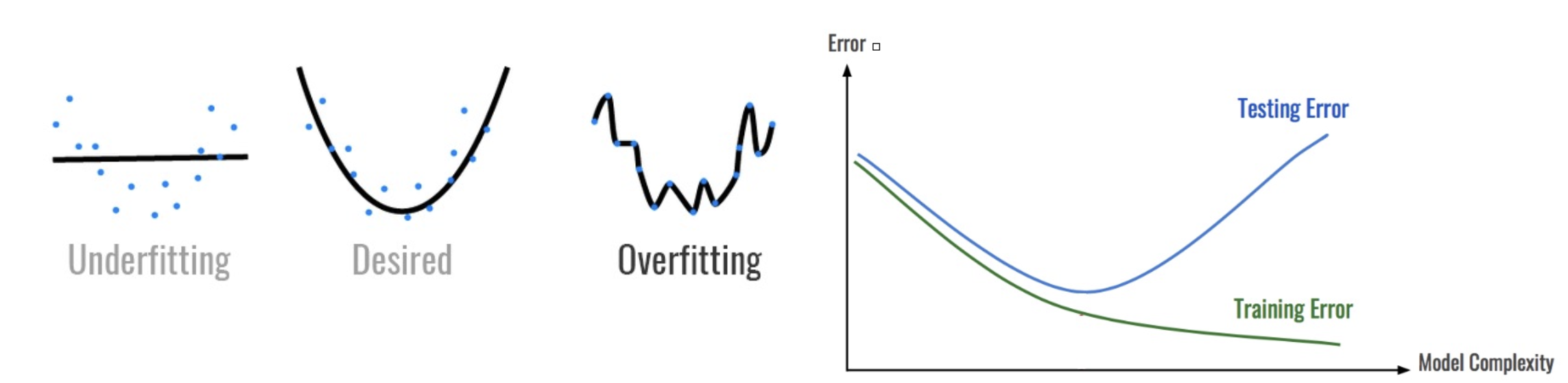
解決辦法:
- early stopping
- stronger regularization
- use more data: data augmentation
- reduce the complexity of model: reduce layer or dropout
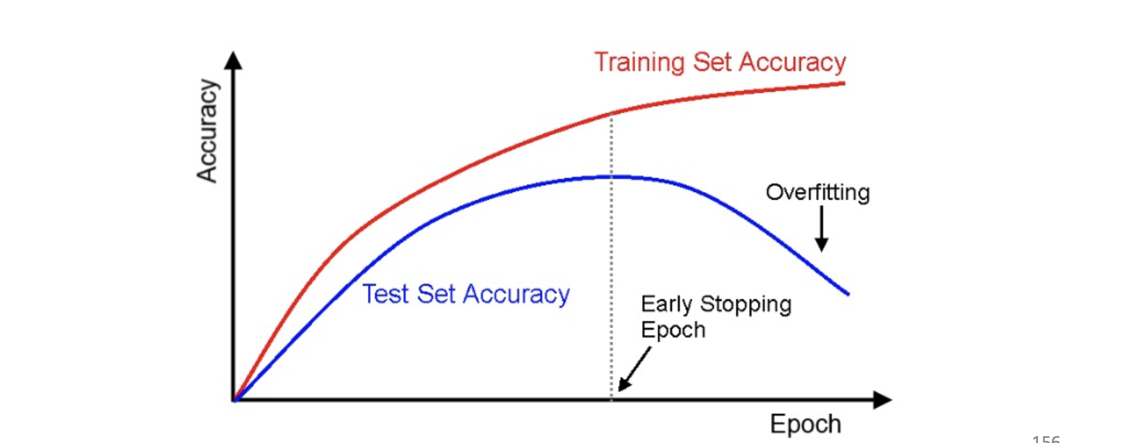
early stopping
- evaluate the accurcy of validation data after every epoch
- when the accuracy becomes stable, stop the training
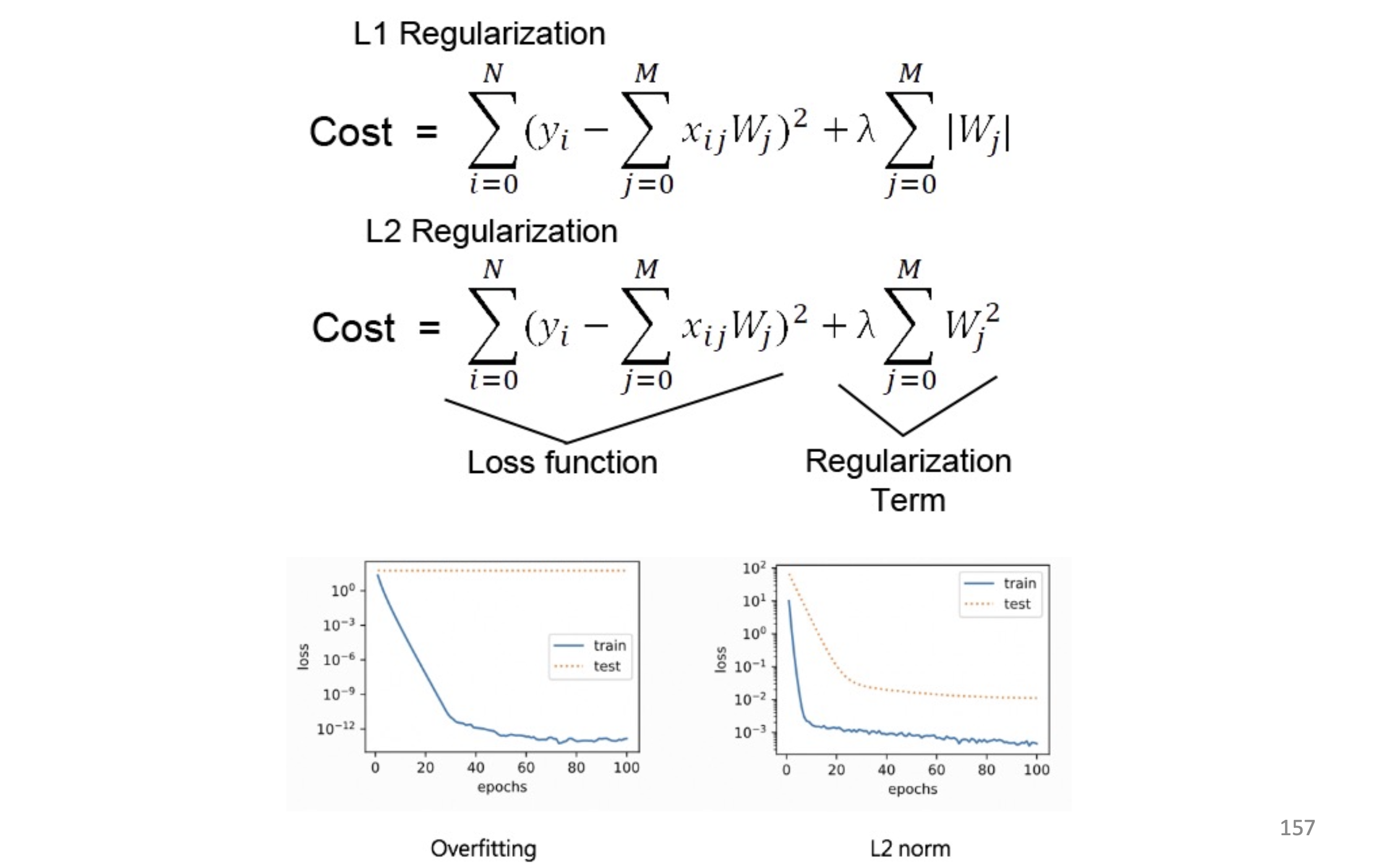
regularization
data augmentation
rotate, crop, resize, change bright…etc to increase the amount of data
reduce the complexity of model
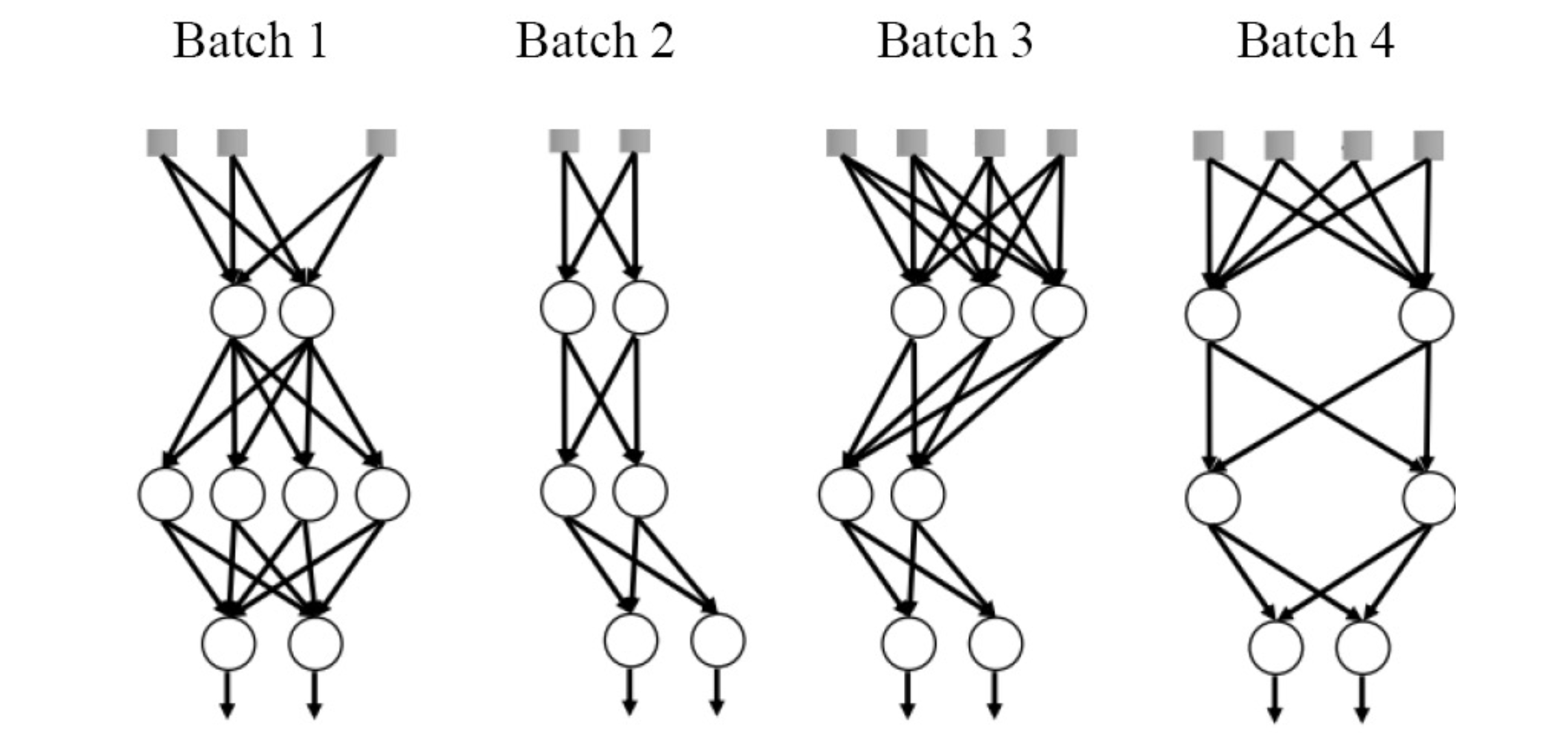
dropout
- when training, each neuron has p% probability dropout(each mini-batch would resample the dropout neuron)
若是對batch size, epoch不是很瞭解的可以前往下面的文章!
機器學習超參數